This page covers the steps used to make and visualize the gaussian cube files created in the ssRNA Example SASSIE Workflow using the Density Plot module. This example uses VMD 1.9.2 but should be nearly the same for older versions.
It is useful to carry out this example to first familiarize yourself with VMD.
We will make the density plots for the ssRNA trajectories that represent 1) all of the accepted structures and 2) only the structures that fit the corresponding SAXS data with x2 < 0.5. This example assumes you are logged into SASSIE-web and you are in a project called test.
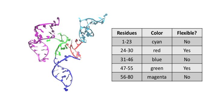
Recall the starting structure:
For density plots, we will define only 3 regions:
The following links allow you to download the files that were created in the ssRNA Example SASSIE Workflow.
Select the 'Analyze' button from the Main Menu of SASSIE-web and then click on the 'Density Plot' button.
You should now see a page like the one below.
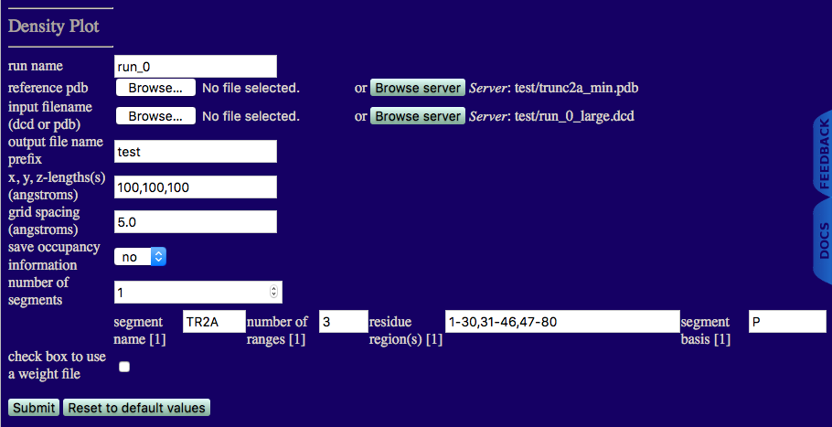
run name: run_0
reference pdb: trunc2a_min.pdb
input filename (dcd or pdb): run_0_large.dcd
output file name prefix: Unique output file name.
x,y,z-length(s) (angstroms): Estimate of the size of overall cube to contain your molecule. Note, box will re-size to fit all structures in your trajectory if the input values are too small.
grid spacing (angstroms:) Cubic length of each voxel.
save occupancy information: Choose to keep non-normalize occupancy values for each voxel.
number of segments: 1
segment name: TR2A
number of ranges: 3
residue region(s): Residue numbers defining each region in segment. The number of pairs should match the number of regions for the given segment. Pairs of integers separated by hypens with each pair separated by commas.
segment basis: Name of the atom to use to determine if a voxel is occupied.
Note that P is used here because each RNA base has a phosphate atom.
check box to use a weight file
This box is not checked since our DCD file represents all accepted structures.
Once you have understood the input fields and made sure that your values agree with the figure click on the 'Submit' button.
Once complete you should see outputs similar to those below.
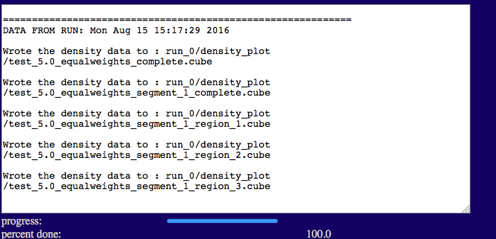
The output will indicate the list of files that were written to disk.
Output file naming
The general recipe is:
"output file name prefix_"grid spacing"_"weight file flag"_segment_"segment number"_region_"region number".cube
In this example:
output file name prefix: test
grid spacing: 5.0
equal weight file not used: equalweights
1 segment in molecule: 1
3 regions in segment: region_1
region_2
region_3
This allows one to experiment with different conditions and keep similar files organized.
test/run_0/density_plot
The following links allow you to download the weight file that was created in the ssRNA Example SASSIE Workflow.
Select the 'Analyze' button from the Main Menu of SASSIE-web and then click on the 'Density Plot' button.
You should now see a page like the one below.
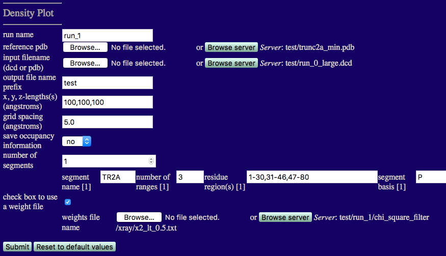
run name: Since we already have a densityplot directory in run0, set this value to run_1.
reference pdb: trunc2a_min.pdb
input filename (dcd or pdb): run_0_large.dcd
output file name prefix: Unique output file name.
x,y,z-length(s) (angstroms): Estimate of the size of overall cube to contain your molecule. Note, box will re-size to fit all structures in your trajectory if the input values are too small.
grid spacing (angstroms): Cubic length of each voxel.
save occupancy information: Choose to keep non-normalize occupancy values for each voxel.
number of segments: 1
segment name: TR2A
number of ranges: 3
residue region(s): Residue numbers defining each region in segment. The number of pairs should match the number of regions for the given segment. Pairs of integers separated by hypens with each pair separated by commas.
segment basis: Name of the atom to use to determine if a voxel is occupied.
Note that P is used here because each RNA base has a phosphate atom.
check box to use a weight file
This box IS checked since our DCD file represents all accepted structures and we want to select only those structures for which x2 < 0.5.
Once you have understood the input fields and made sure that your values agree with the figure click on the 'Submit' button.
Once complete you should see outputs similar to those below.
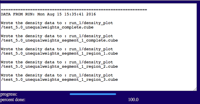
The output will indicate the list of files that were written to disk.
test/run_1/density_plot
The following links allow you to download the files created above that will be needed for this exercise.
test_5.0_equalweights_segment_1_region_1.cube
test_5.0_equalweights_segment_1_region_2.cube
test_5.0_equalweights_segment_1_region_3.cube
test_5.0_unequalweights_segment_1_region_1.cube
test_5.0_unequalweights_segment_1_region_2.cube
test_5.0_unequalweights_segment_1_region_3.cube
Open VMD.
Select File -> New Molecule... and load the test_5.0_equalweights_segment_1_region_1.cube file.
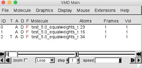
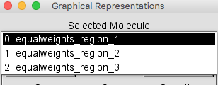
Do the same for the test_5.0_equalweights_segment_1_region_2.cube and test_5.0_equalweights_segment_1_region_3.cube files. Be sure to choose New Molecule each time. Your VMD Main window should look like the one below.
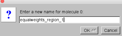
Since the file names are long, it is difficult to tell which cube file is associated with each molecule ID number. Select the first molecule (ID 0) and double-click on the file name. A small window will open that will allow you to edit the file name.
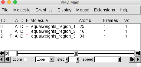
Do the same for the other two molecules. The VMD Main window should now look like this.
Select Graphics -> Representations... to open the Graphical Representations window. Select the molecule with ID value 0, corresponding to region 1, from the Selected Molecule pull-down menu.
Then, for the Drawing Method option choose Isosurface. This should give you the following window.
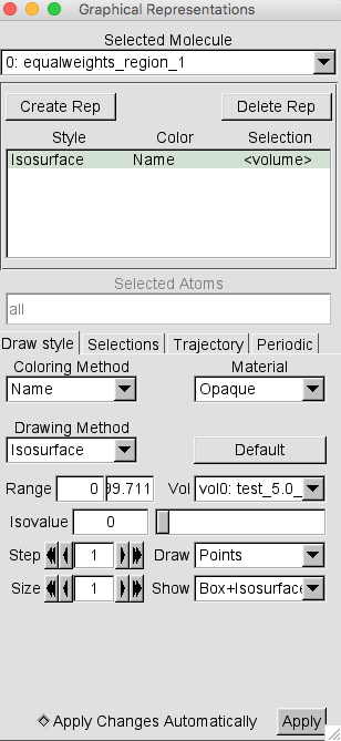
Note that the default settings are to Draw Points and Show Box+Isosurface. Change these settings to Wireframe and Isosurface respectively.
Then change the Isovalue from the default 0 to 0.01 and press RETURN. This is a reasonalbly low value to capture the complete volumetric data set.
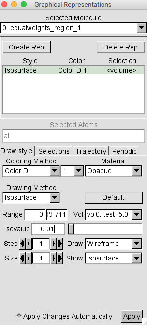
Then change the Coloring Method to Color ID and select 1 as the option.
Your Graphical Representations window should look similar to this.
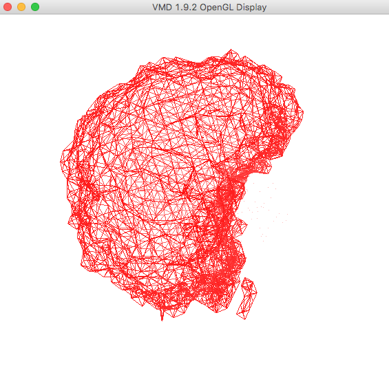
From the VMD Main window, select Display -> Axes -> Off.
The plot in the OpenGL Display window , once re-oriented for visual purposes, is shown below.
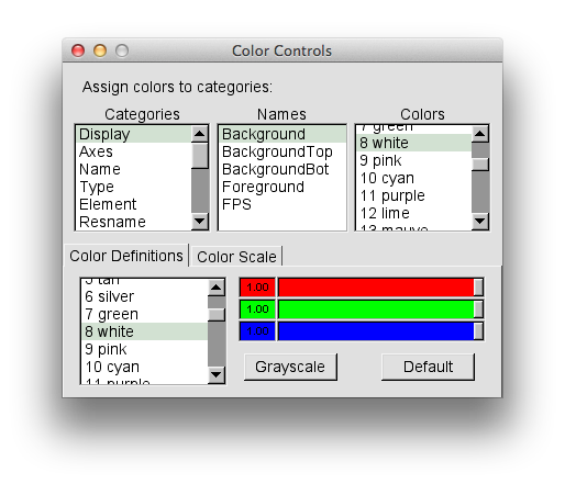
Your version will probably have a black background. To switch the color of the background to white, choose Graphics -> Colors.... Select Display in the Catagories section, Background in the Names section, and 8 white in the Colors section, as shown in the picture below.
To display the other two regions, repeat the last few steps above for the molecules with ID values 1 and 2, corresponding to regions 2 and 3, respectively. Start with the selection of each molecule from the Selected Molecule pull-down menu, then change the Drawing Method and Coloring Method in each case as described above. Choose a Color ID value of 0 for molecule 1 and a Color ID value of 7 for molecule 2.
Note: When loading multiple gaussian cube files, as shown below, make sure that the Isovalue setting is the same for all files, otherwise the visulaization may be misleading.
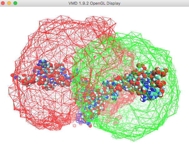
The plot in the OpenGL Display window , once re-oriented for visual purposes, is shown below.
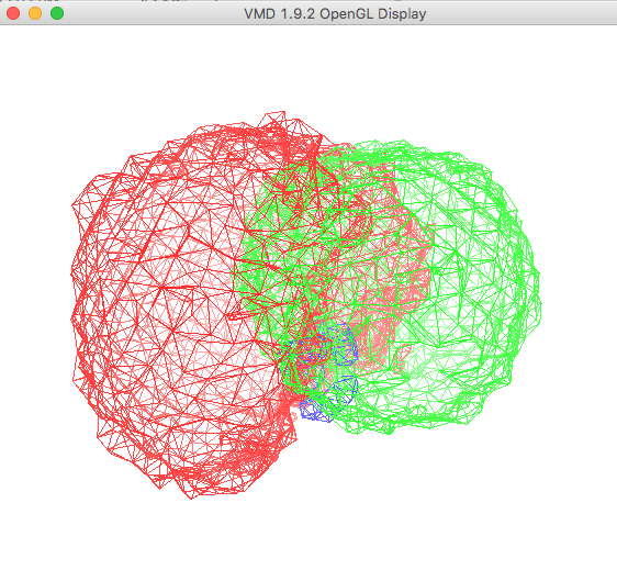
At this point you are displaying the region of three-dimensional space for all structures that were accepted from the ssRNA Example SASSIE Workflow.
In this section the original structure along with the accepted structures from the simulation will be loaded into a new molecule in the same VMD session described above.
Select File -> New Molecule... and load the trunc2a_min.pdb. Then, in the same Molecule File Browser load the trajectory from run_0_large.dcd. DO NOT choose New Molecule in this case. Your Molecule File Browser should look like the one below.
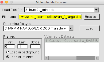
NOTE It is faster to select the "Load all at once" option in the Molecule File Browser when loading a large trajectory. This sidesteps the animation of each frame as the trajectory loads.
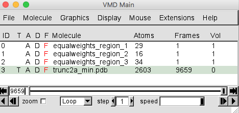
Once the trajectory is loaded your VMD Main window should look like this.
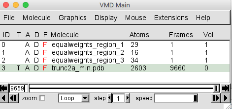
The trajectory contains 9659 frames. The trunc2a_min.pdb entry in the Molecule File Browser will indicate that there are 9660 frames loaded. This is because the PDB of the starting structure was loaded before the trajectory. That original structure may or may not have been accepted. So for completeness, this single frame should be removed.
NOTE: VMD counts frames starting at 0, not 1.
To remove frame 0, the coordinates from the starting PDB file, select the Molecule -> Delete Frames.... Then in the Frame Selector pop-up window change the value of the Last frame from 9659 to 0 as shown on the right side of the image below.
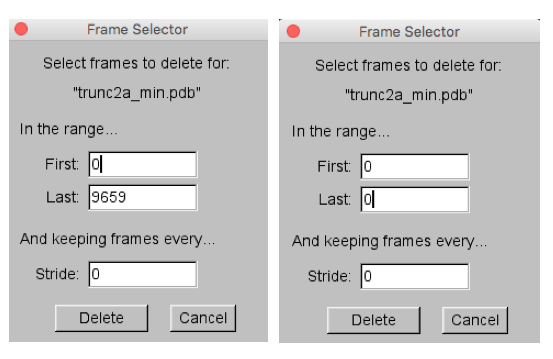
Then hit the Delete button to complete the task. The VMD Main Menu should now indicate that only 9659 frames are in the trunc2a_min.pdb molecule.
In the Open GL window, it may be difficult to see the protein structure. In the Graphical Representations window, select VDW in the Drawing Method option box. This will give you something similar to the view below.
Use the slider to examine the trajectory frames to see how the density plot represents the region of conformation space occupied by the accepted structures.
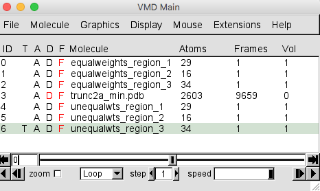
Choose File -> New Molecule and load the test_5.0_unequalweights_segment_1_region_1.cube file.
Do the same for the test_5.0_unequalweights_segment_1_region_2.cube and test_5.0_unequalweights_segment_1_region_3.cube files. Be sure to choose New Molecule each time. Shorten the names for your newly-loaded molecules. Your VMD Main window should look like the one below.
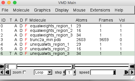
At this point, we won't need to visualize the trajectory of all accepted structures. In the VMD Main menu, select molecule 3, corresponding to the trajectory, and click on the D next to the file name to toggle the display off. The D will now appear in red as shown below and the trajectory will no longer be displayed in the OpenGL Display window.
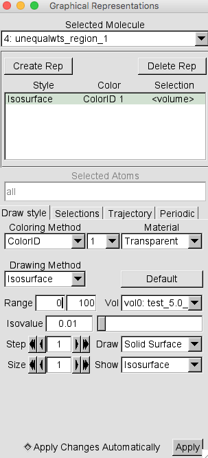
Select Graphics -> Representations to open the Graphical Representations window. Select molecule 4, corresponding to region 1 for the structures with x2 < 0.5, from the Selected Molecule pull-down menu. Then, for the Drawing Method option choose Isosurface.
Again, note that the default settings are to Draw Points and Show Box+Isosurface. This time, change these settings to Solid Surface and Isosurface respectively. Also, change the Material option from Opaque to Transparent.
If necessary, change the Isovalue to 0.01 and press RETURN. Then change the Coloring Method to Color ID and select 1 as the option.
Your Graphical Representations window should look similar to this.
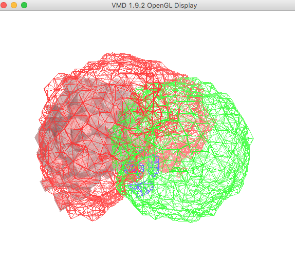
From the VMD Main window, choose Display -> Rendermode -> GLSL. Then select Display -> Axes -> Off.
The plot in the OpenGL Display window , once re-oriented for visual purposes, is shown below.
To display the other two regions, repeat the last few steps above for molecules 5 and 6, corresponding to regions 2 and 3 for the structures with x2 < 0.5, respectively. Start with the selection of each molecule from the Selected Molecule pull-down menu, then change the Drawing Method, Material and Coloring Method in each case as described above.
Leave the Material setting on Opaque for molecule 5, which corresponds to region 2.
Choose a Color ID value of 0 for molecule 5 and a Color ID value of 7 for molecule 6. The plot in the OpenGL Display window , once re-oriented for visual purposes, is shown below.
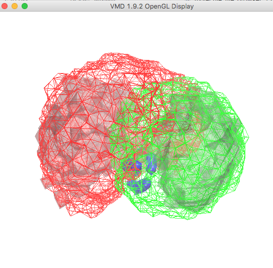
At this point you are displaying the regions of three-dimensional space for all structures that were accepted (mesh) as well as the regions for those structures with x2 < 0.5 (transparent solid) from the ssRNA Example SASSIE Workflow. Note that region 2 (opaque solid) is the same in both cases.
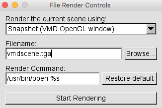
The images produced using VMD can be saved by choosing File -> Render.... This will open the File Render Controls window. You can render the current scene using the default method to take a screen shot of the VMD OpenGL Window. The default picture type depends on the operating system. It is "tga" for OS-X as shown in the figure below.
Select Browse... before rendering the picture in order to choose the direcory where you want to save the picture as well as the picture name. You can use the default Render Command. To render the picture, Press Start Rendering.
You can also save the VMD state by writing a text file containing all of the instructions that were executed in the current VMD session by choosing File -> Save Visualization State... in order to save a state file. The default extension is "vmd". This state file can be loaded upon opening a new session of VMD to restore VMD back to the exact state that was saved. This is done by choosing File -> Load Visualization State.... Note that VMD state won't be restored properly if the structure files are moved to a different directory than the one that was recorded in the state file. However, since these files are text files, they can be edited to change the file path to the new location so that the state files will work properly again.
VMD - Visual Molecular Dynamics W. Humphrey, A. Dalke, K. J. Schulten, Molec. Graphics, 14, 33-38 (1996). BIBTeX, EndNote, Plain Text
SASSIE: A program to study intrinsically disordered biological molecules and macromolecular ensembles using experimental scattering restraints J. E. Curtis, S. Raghunandan, H. Nanda, S. Krueger, Comp. Phys. Comm. 183, 382-389 (2012). BIBTeX, EndNote, Plain Text