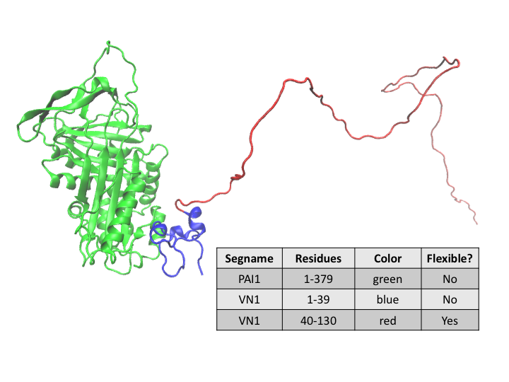
In this workflow example we will model the conformation of a disordered region of the glycoprotein vitronectin (VN) that is in a complex with plasminogen activator inhibitor-1 (PAI-1). PAI-1 inhibits the activation of plasminogen to plasmin, which has a key role in fibrin degradation, Extra Cellular Matrix remodeling and cell migration. Binding of its co-factor, VN, stabilizes PAI-1 so that it can perform its function. Residues 1-39 of VN are structured when bound to PAI-1. However, residues 40-130 of VN remain disordered.
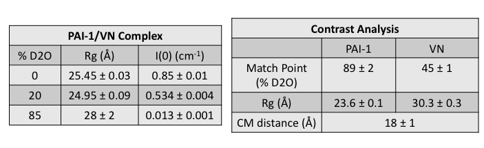
The complex that was measured on the EQ-SANS instrument at Oak Ridge National Lab using contrast variation consists of one subunit of 60% deuterated PAI-1 in complex with one subunit of protonated VN. The Contrast Calculator module was used prior to the SANS experiment to determine that the match point of the complex occurs in 77% D2O buffer. The match point of the deuterated PAI-1 occurs in 88% D2O buffer (and that of VN in 44% D2O buffer). The complex was measured at a concentration of about 8 mg/ml in 0%, 20% and 85% D2O buffers. In 85% D2O buffer, the scattering from PAI-1 is negligible compared to that of VN.
An initial structure was built from a co-crystal structure (PDB ID 1OC0) of PAI-1/VN(1-39) with VN(40-130), along with other missing residues, added. The initial structure was energy-minimized and subjected to a short SASSIE Complex Monte Carlo run to obtain the "starting" structure shown above.
After calculating Rg and I(0) for the data at each contrast, the match point, Stuhrmann and parallel axis theorem analyses were performed using MulCh. The pertinent results that are needed for this analysis are shown below.
NOTE: This work was part of the thesis of Letitia N. Puster. The example presented here begins from just one of several starting structures that were explored for this complex. The other starting structures considered the possibility that residues 40-130 contained some ordered regions, such as helices. Only a relatively small number of structures are generated in this example for illustration purposes. A real study typically requires 10,000 to 50,000 accepted structures to adequately sample configuration space.
In this example it is assumed that the sassie-web project name is test. Download the PAI-1 and VN sequences and the starting structure files pai_vn_start.pdb and pai_vn_start.psf to visualize the starting structure and perform the contrast calculations, PDB Scan and Monte Carlo analysis in this example. The data are not provided at this time since the manuscript is still in preparation. Substitute your own files to go through the entire example with your contrast variation data.
Here we demonstate the use of the Contrast Calculator module to aid in experiment planning. More information on the Contrast Calculator module is available in the Contrast Calculator documentation.
Select the 'Contrast Calculator' button from this 'Tools' menu. You should now see a page like the one below. This page is used to enter all of the information needed to calculate the SANS scattering length densities, contrasts and I(0) values for PAI-VN in H2O:D2O buffers.
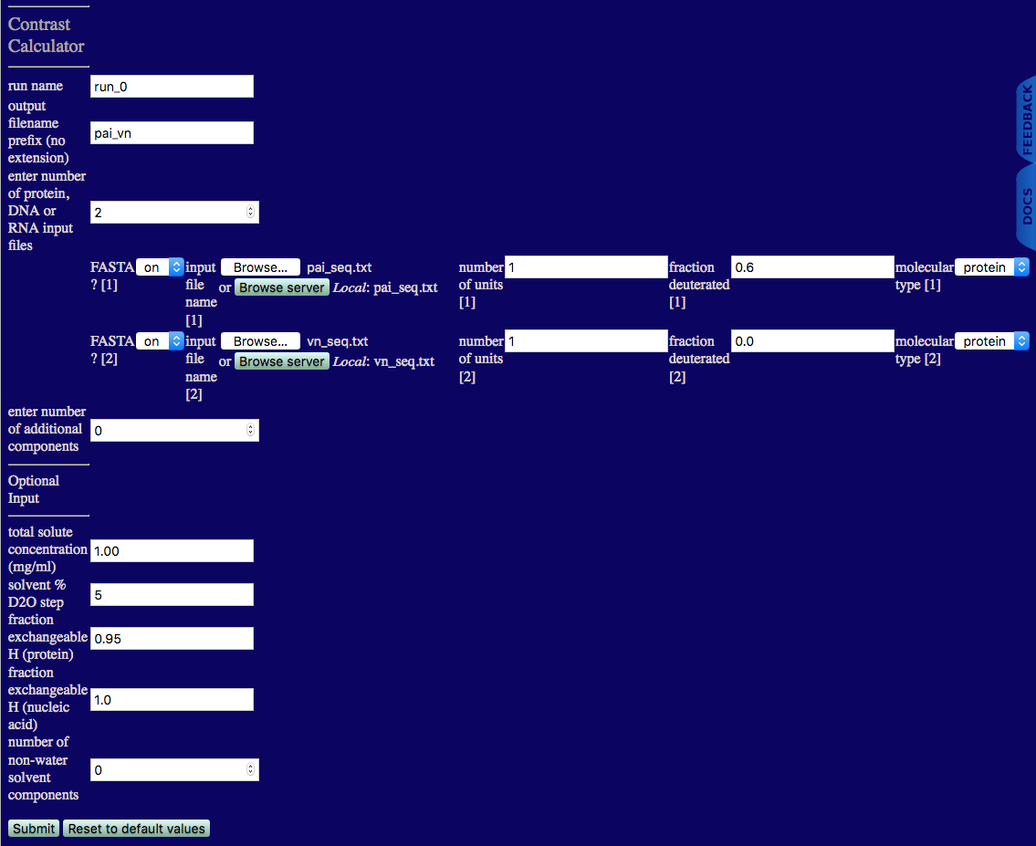
number of protein, DNA or RNA input files: The number of FASTA and/or PDB files that will be used in the complex. In this case, there is one file for PAI and one for VN, so the number of protein, DNA or RNA input files is 2. Additional information regarding the input files then must be provided as follows.
number of additional components: The number of additional components in the complex that are not protein, DNA or RNA, such as polymers, lipids, carbohydrates, etc. If this number is not zero, then additional input fields will be provided to enter the desired chemical formula, mass density and other pertinent information. (If the number of protein, DNA or RNA input files is 0, then this number cannot be 0.)
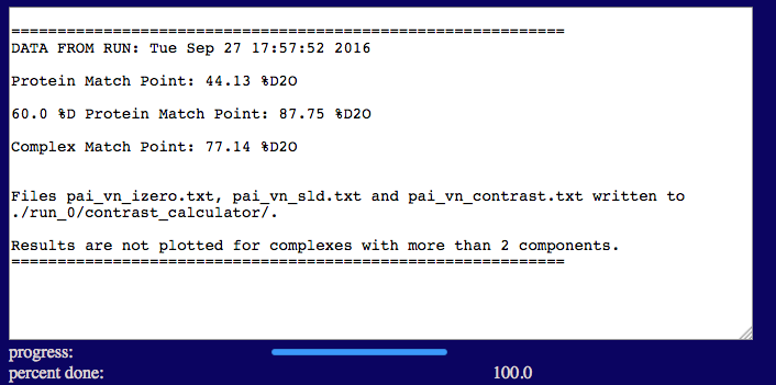
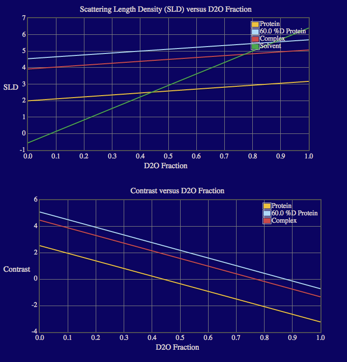
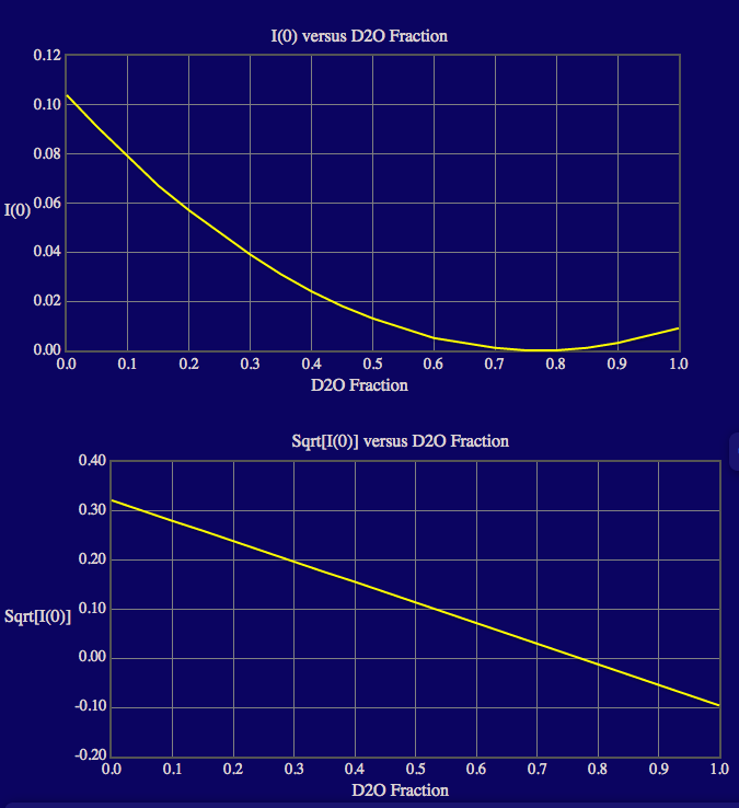
The output screen lists the match points for the protein and 60% deuterated protein components in the complex as well as for the entire complex. The output also shows plots of the calculated neutron SLDs, contrasts, I(0) and sqrt[I(0)] as a function of % D2O in the solvent since the complex doesn't contain more than 2 components. Note that roll-over help will indicate options to resize, zoom and reset the view of the plots. Resultant files containing the SLD, contrast and I(0) values are written to a new directory, "contrast_calculator", within the run_0 directory.
 <-
->
<-
-> <-
->
<-
->
test/run_0/contrast_calcuator
Data interpolation is necessary to create a new data file that is spaced on a uniform grid from the experimental data file. The number of q-points, range of q, and the spacing of the q-points used to create the interpolated data files MUST match the input settings that you use in subsequent modules to calculate SAS profiles that are subsequently used to compare theoretical and experimental data. The interpolation must be performed for the data at all contrasts measured.
Since the data are not provided for this example, the data interpolation is not shown here. For an example of how to interpolate your own data, please refer to the Data Interpolation documentation.
The PAI-VN data were interpolated as follows:
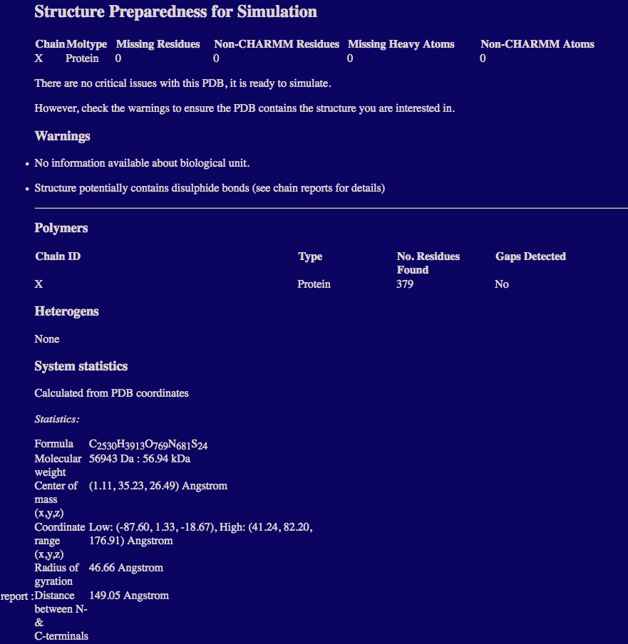
PDB Scan is used to assess whether an input PDB is ready for simulation and where possible to provide files enabling CHARMM forcefield parameterization. Information on missing atoms and residues and those not covered as standard by the CHARMM 27 forcefield are reported. PDB files do not need to have header information. At this time, only PDB files of proteins are supported. More information on the module is available in the PDB Scan documentation.
Select the 'Build' button from the Main Menu of SASSIE-web and then click on the 'PDB Scan' button.
You should now see a page like th one below. This page is used to enter all of the information needed to check the PDB file.
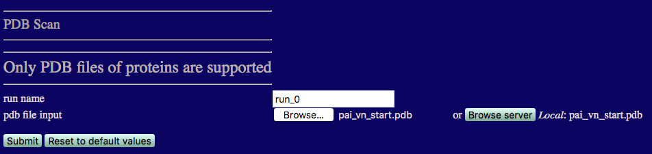
pdb file input: The PDB file that we want to examine. Here we use the pai_vn_start.pdb file.
Once you have entered the file name, click on the 'Submit' button to start the file scan.
As the run continues the progress bar beneath the submit button should update. Once complete the output should look similar to the figure below.
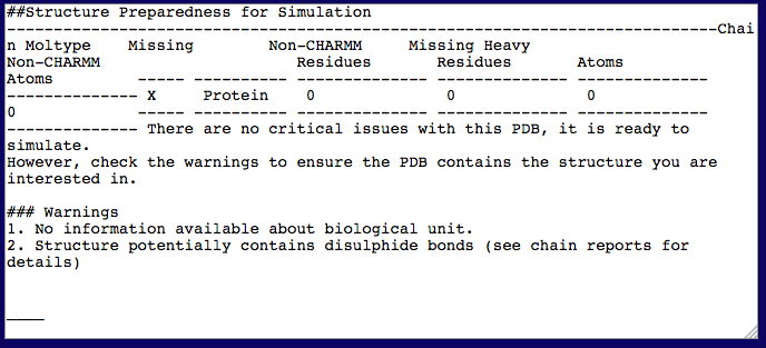
The text output region provides a brief summary of the PDB Scan report.
test/run_0/pdbscan
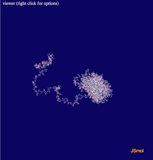
A JSmol vizualization of the protein is produced and is shown below the text output region. Holding down the left mouse button and moving the cursor over the picture allows you to rotate the view, the scroll wheel facilitates zooming in and out. Right clicking on the image allows you to access all of the JSmol options.
The full PDB scan report can be found below the image of the structure.
The pai_vn_start.psf and pai_vn_start.pdb files can also be loaded into VMD or a similar structure viewer to observe the location of the disulphide bonds. This PDB file is ready for simulation so we can proceed to create an ensemble of structures for comparison to the SANS data.
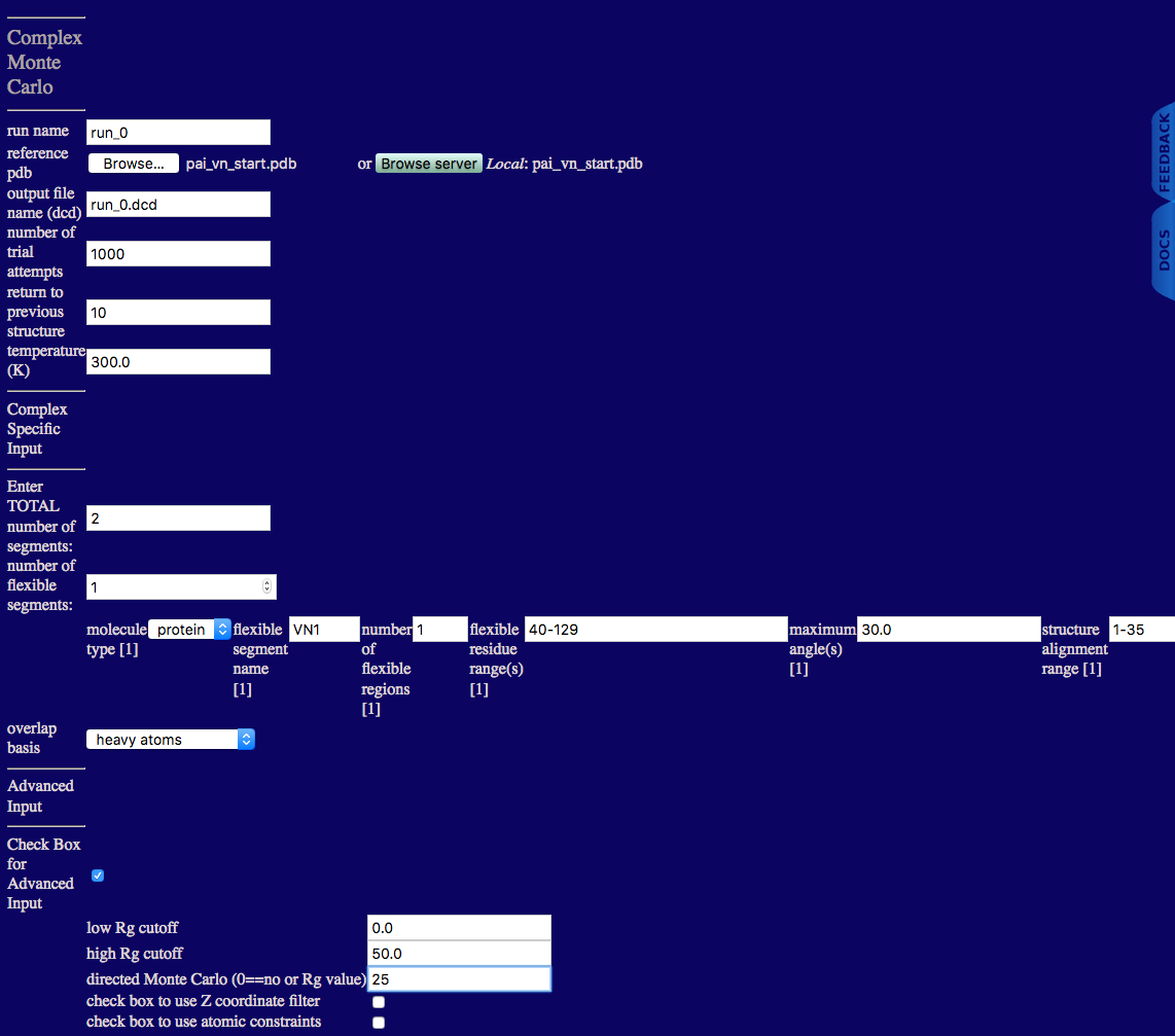
Complex Monte Carlo is used to generate a series of structures to sample configurations of the PAI-VN complex. The single flexible region in the VN subunit is shown in the structure and table above. More information on the module is available in the Complex Monte Carlo documentation.
Select the 'Simulate' button from the Main Menu of SASSIE-web and then click on the 'Complex Monte Carlo' button.
run name: user defined name of folder that will contain the results.
reference pdb: PDB file with naming information and coordinates of the starting structure.
output file name (dcd): Name of ouput DCD file containing accepted structures from the simulation.
number of trial attempts: Number of Monte Carlo moves to attempt.
return to previous structure: After this number of Monte Carlo moves fails to find an accepted configuration, re-load a previously accepted structure.
temperature (K): Simulation temperature.
Enter TOTAL number of segments: An integer value indicating the number of rigid and flexible segments in the input PDB file.
number of flexible segments: An integer value indicating the number of regions to sample backbone torsions.
molecule type: Select protein.
flexible segment name: Name of particular flexible segment .
number of flexible regions: An integer value indicating the number of regions to sample backbone torsions.
flexible residue range(s): Residue numbers defining each flexible region in segment. The number of pairs should match the number of flexible regions for the given segment. Pairs of integers separated by hypens with each pair separated by commas.
maximum angle(s): Angle, in degrees, that can be sampled in a single move for each region.
structure alignment range: Residue to define the beginning of region used to align structures for the given segment.
overlap basis: Select either heavy atoms, all, backbone or enter atom name. The atom name option will spawn futher inputs:
overlap basis: Enter an atom name to check for overlap.
overlap cutoff (angsgtroms): Overlap basis atoms closer than this distance defines an overlap condition.
Here the advanced options are used to set a high Rg cutoff value and to direct the Monte Carlo to a particular Rg value. These values were chosen based on the Rg values obtained from the contrast variation data and from the contrast analysis. The Rg value calculated in this module is the molecular Rg derived from the coordinates. Thus, it DOES NOT depend on the contrast. Therefore, the Rg value is directed to 25 Å, which is close to the experimental values obtained in 0% and 20% D20. These are the contrasts that we want to refer to when deciding on the directed Rg value since the molecular Rg always includes both subunits. PAI doesn't contribute to the scattering in 85% D2O, so we don't want to direct the molecular Rg to this experimental Rg value.
low Rg cutoff: Structures with Rg values less than this value are discarded.
high Rg cutoff: Structures with Rg values greater than this value are discarded.
directed Monte Carlo (0==no or Rg value): Enter a non-zero value to use an extra energy term in the Monte Carlo sampling to favor Rg values towards the supplied value. The default value is zero which indicates that no bias is implemented.
check box to use Z coordinate filter: Check box to implement the ability to discard structures with any Z coordinates with a value less than the user supplied Z cutoff value.
check box to use atomic constraints: Check box to implement the ability to discard structures that do not satisfy the atomic / geometric constraints provided in the user defined constraint file.
Once complete the output should look similar to the figure below.
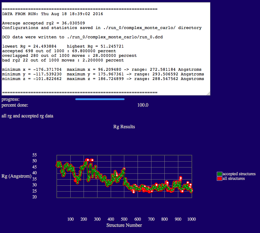
The output will indicate various Rg values from the ensemble, acceptance and overlap statistics, and dimensions of the accepted structures in the final ensemble.
Results are written to a new directory within the given "run name" as noted in the output. In addition, a plot of Rg versus structure number is shown.
Several files are generated and saved to the "run name" complex_monte_carlo directory. A copy of the original input PDB file, the output DCD file containing accepted structures, files with Rg values as shown in the plot on the web-page, and run statistics.
test/run_0/complex_monte_carlo
REMINDER: This example has only 698 accepted structures. For a real study, 10,000 to 50,000 accepted structures would be needed to adequately cover configuration space.
We will use SasCalc to calculate the SANS curves from the generated structures. More information can be found in the SasCalc documentation. The starting structure must be a complete structure without missing residues or atoms (including hydrogen atoms) in order to obtain accurate scattering profiles. Atom and residue naming must be compatiable with those defined in the CHARMM force field.
The SasCalc module is first run using the "converged number of golden vectors" option on just one structure. We will calculate the SANS curves at each contrast for the PAI-VN starting structure. In order to create theoretical curves with data points at q values that match our interpolated data, we need three pieces of information:
Select the 'Beta' button from the Main Menu of SASSIE-web and then click on the 'SasCalc' button.
Since this is the first time we are running SasCalc on this structure, we are using the "converged number of golden vectors" option. The scattering profile is calculated several times using an increasing number of golden vectors until there is no difference between the calculated scattering curves to within a chosen tolerance (averaged over the entire scattering profile). This is useful for determining the fixed number of golden vectors that are needed to achieve convergence within a chosen tolerance. The smaller the tolerance value specified in the converged option, the smaller the differences in the scattering profiles over the entire q range specified. In this case, a tolerance of 0.001 has been chosen.
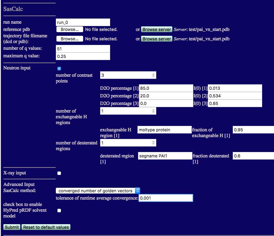
The single structure that we used to start the simulation is used as both the reference pdb and the trajectory file filename (PDB in this case) so it is already uploaded to the SASSIE-web server. Thus, you can either upload it again from your local computer or locate it on the server and read it from there.
Note that we are calculating the SANS curves for all three contrasts at the same time. The number of exchangeable H regions is 1 since the H-D exchange is the same for both protein subunits. Thus, the exchangeable H region can be set to "moltype protein" and the fraction of exchangeable H value is set to 0.95. Only the PAI-1 subunit is deuterated, so the number of deuterated regions is 1. The deuterated region can be specified using "segname PAI1" and the fraction deuterated is set to 0.6. Once the calculations are finished, the output will look similar to the figure below.
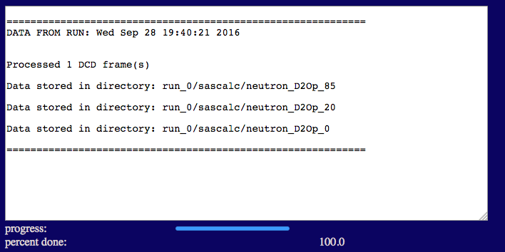
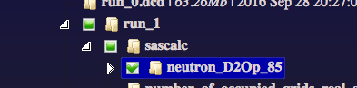
The output files are written to a sub-directory of sascalc/ that is named according to the D2O percentage in the solvent.
test/run_0/sascalc/neutron_D2Op_85
Similarly, we have:
test/run_0/sascalc/neutron_D2Op_20
test/run_0/sascalc/neutron_D2Op_0
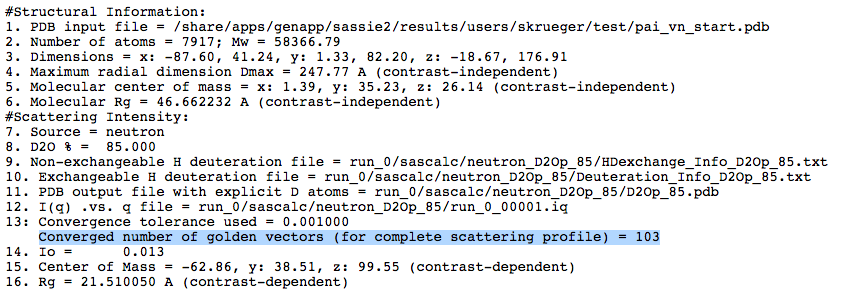
Next we calculate a theoretical scattering curve for each of the trial structures we have generated for the contrast condition in 85% D2O. We are interested in the best fitting structures at all contrasts. However, since the PAI-1 structure is fixed, we want to narrow down the structures that fit the VN portion of the complex and then compare that subset of structures to the entire contrast variation data set to extract the best structures that fit all of the data. The run_0_00001.log files from the inital SAS Curve calculation at each contrast indicate that 103, 73 or 83 golden vectors were required for convergence to the desired tolerance (0.001 in this case) for 85%, 20% and 0% D2O, respectively. The log file for 85% D2O is shown below.
We now use this information to calculate the scattering curves for all of the generated structures using the "fixed number of golden vectors" option from the SasCalc method menu as shown below.
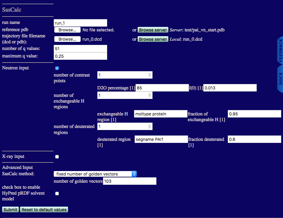
run name: run_1 to avoid overwriting the files we calculated in run_0 above
reference pdb: the starting structure that is already on the SASSIE-web server
trajectory file filename: the run_0.dcd file generated using Complex Monte Carlo
Once the calculations are finished, the output will look similar to the figure below.
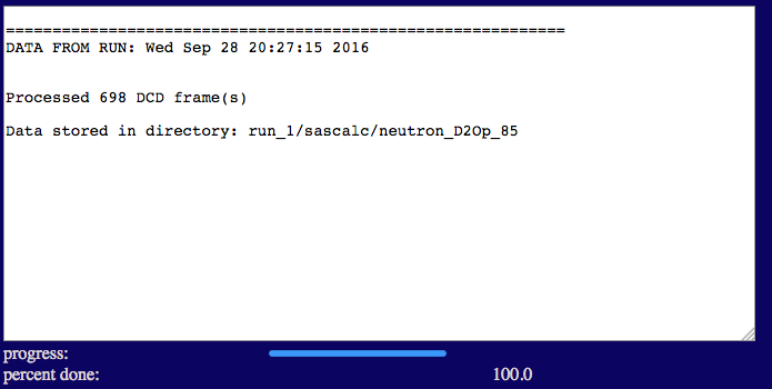
test/run_1/sascalc/neutron_D2Op_85
Now we compare our theoretical curves to the experimental data taken in 85% D2O using Chi-Square Filter. More information can be found in the Chi-Square Filter documention.
Select the 'Analyze' button from the Main Menu of SASSIE-web and then click on the Chi Square Filter button.
The inputs are shown in the figure below.
Note that you are required to select the path on the server containing the theoretical scattering curves, i.e., they can't be uploaded from your local computer. To set the path to the scattering curves generated in the previus step:
I(0) must match that from the 85% D2O data: 0.013
number of weight files Set this to 0 since we don't know what x2 and Rg values exist until we perform this first comparison.
Check the box for Advanced Input and then check the box to keep existing run folder name. This will put the output in a directory under chi_square_filter that matches the path that you chose above, i.e., chi-square_filter/neutron_D2Op_85, so that it isn't overwritten when comparing data at more than one contast.
Once complete you should see outputs similar to those below.
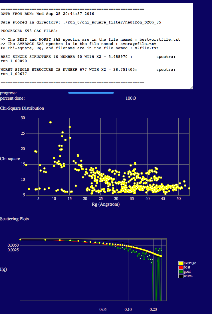
In the text output you will see the minimum chi square (X2) values is given.
The top plot shows the variation of chi squared (y-axis) with the radius of gyration (x-axis).
NOTE that the Rg values in the plots are the scattering Rg values (calculated in SasCalc) and they are contrast-dependent! The low Rg values (< ~20 Å) are due to the fact that the disordered tail (40-130) of VN is so long that portions are interacting with its ordered, fixed region (1-39). (Remember that PAI-1 is not visible at this contrast!) Thus, there is no longer a true Guinier region due to this intra-particle interaction. This results in a depressed I(0) value and a lower apparent Rg. In some cases, a weak intra-particle interaction peak can even be observed in the scattering curves such that the Guinier region is undefined. In these cases, Rg is listed as "nan" in the output file. This will not occur in every system. It occurs at this contrast in this system since VN has a long disordered tail region compared to the size and mass of its ordered region. Thus, in some configurations, the two regions of VN essentially act as if they were separate particles (like two ends of a barbell) and can interfere with each other.
The bottom plot shows a direct comparison of the best, worst and average theoretical curves with experiment (goal).
test/run_1/chi_square_filter/neutron_D2Op_85
/spectra
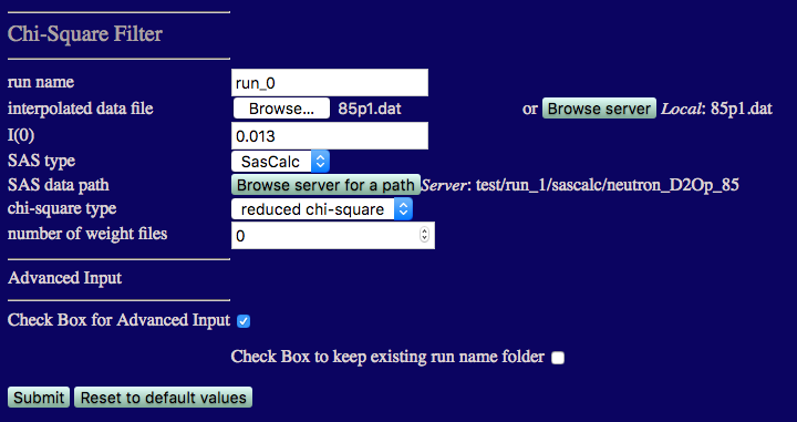
Now that we know the range of chi square values that we have, we can compare the theoretical curves to the data a second time and create a weight file that flag all structures with chi square and Rg values in a desired range. Now, we set the 'number of weight files' to 1.
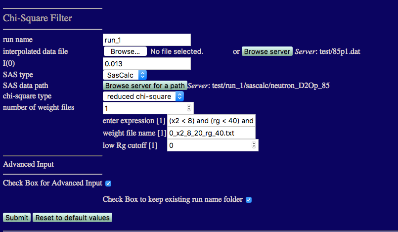
run name: Since we already have a chi_square_filter folder in the run_0 directory, set the run name to run_1.
number of weight files: Set this to 1 using the down arrow associated with the input box.
Weight files contain information on which frames in our simulation meet specific criteria provided in the expression box.
enter expression[1]:
(x2 < 8) and (rg < 40) and (rg > 20)
Adjust these values if necessary to suit the results from your simulation.
weight file name[1]:
low Rg cutoff[1]:
Once complete the outputs should be exactly the same as for the previous run. The only difference is that the a weight file can now be found in the chi_square_filter/neutron_D2Op_85 folder.
test/run_1/chi_square_filter/neutron_D2Op_85
/spectra
Now we can filter out the best fit structures and vizualize them using the Extract Utilities. More information can be found in the Extract Utilities documentation.
We will extract the frames from run_0.dcd that fit the data with x2 < 8 and Rg between 20 Å and 40 Å.
Select 'Tools' from the Main Menu and click the 'Extract Utilities' button.
Check the tick box labelled 'extract trajectory' to reveal the options shown in the figure below.
NOTE: 'extract SAS' is not yet implemented for SasCalc output.
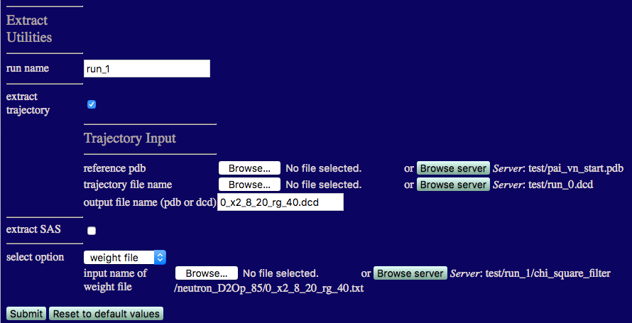
output filename: Enter 0_x2_8_20_rg_40.dcd
Choose 'weight file' from the 'select option' listbox.
When the process is finished your output should look like the one below.
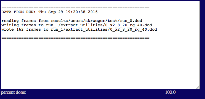
test/run_1/extract_utilities
Next we calculate a theoretical scattering curve at all contrasts for each of the trial structures that we extracted above. We will use the "fixed number of golden vectors" option from the SasCalc method menu as shown below. We choose 103 golden vectors for all contrasts since that is the largest number of golden vectors we found were necessary to converge the calculated scattering curves to a tolerance of 0.001.
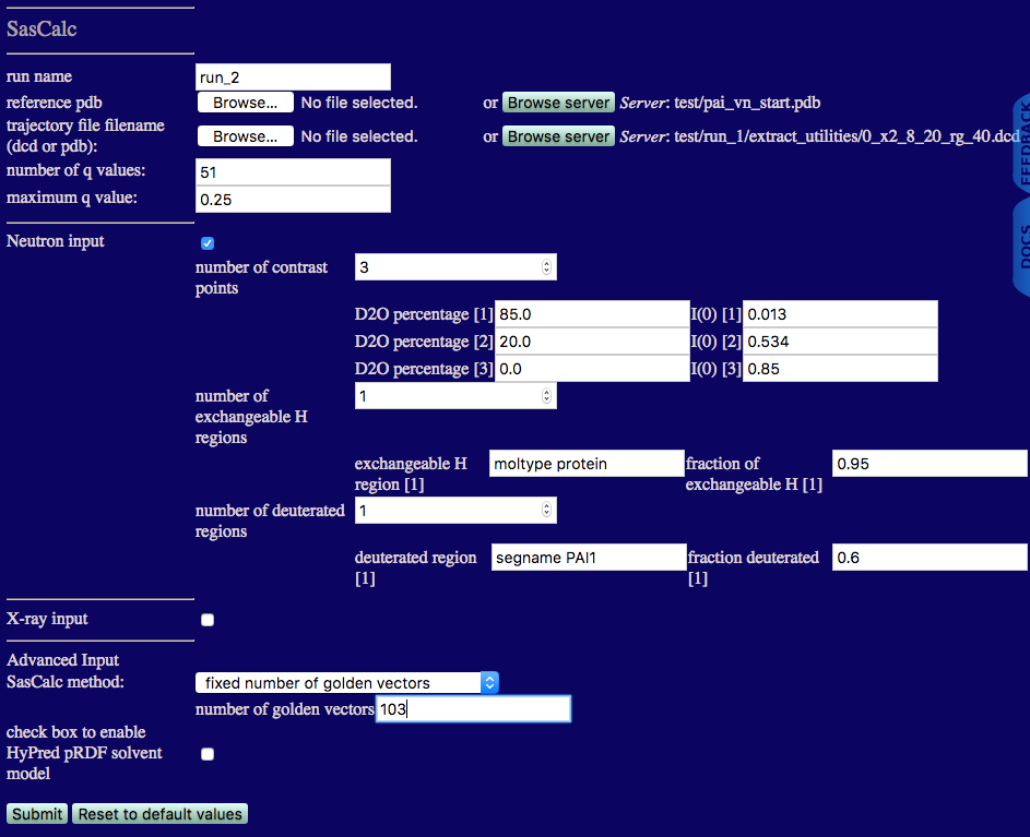
run name: run_2 to avoid overwriting the files we calculated in run_1 above
reference pdb: the starting structure that is already on the SASSIE-web server
trajectory file filename: the 0_x2_8_20_rg_40.dcd file that we just extracted
Once the calculations are finished, the output will look similar to the figure below.
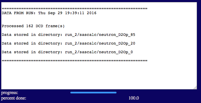
test/run_2/sascalc/neutron_D2Op_85
test/run_2/sascalc/neutron_D2Op_20
test/run_2/sascalc/neutron_D2Op_0
Now we compare our theoretical curves to the experimental data taken at all 3 contrasts using Chi-Square Filter. More information can be found in the Chi-Square Filter documention.
We start with the 85% D2O case. The inputs are shown in the figure below.
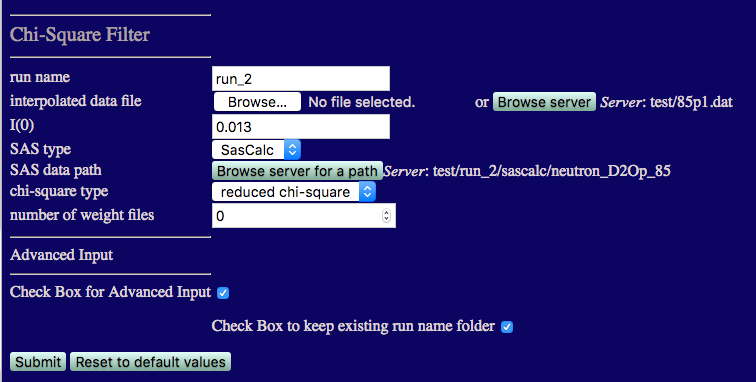
run name run_2 to avoid overwriting earlier calculations
I(0) must match that from the 85% D2O data: 0.013
number of weight files Set this to 0 since we don't know what x2 and Rg values exist until we perform this first comparison.
Check the box for Advanced Input and then check the box to keep existing run folder name. This will put the output in a directory under chi_square_filter that matches the path that you chose above, i.e., chi-square_filter/neutron_D2Op_85, so that it isn't overwritten when comparing data at more than one contast.
Once complete you should see outputs similar to those below.
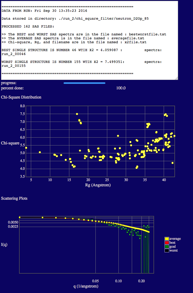
In the text output you will see the minimum chi square (X2) values is given.
The top plot shows the variation of chi squared (y-axis) with the radius of gyration (x-axis).
NOTE that there are some additional low Rg values (< ~20 Å) present. Each time the SANS curves are calculated, the deuteration of exchangeable and non-exchaneable hydrogen atoms is random. At this contrast (where PAI-1 is not contributing to the scattering), for those structures that have Guinier regions with nearly flat or negative slopes, a small change in the location of the deuterated hydrogen atoms can cause a relatively large change in calculated Rg. These structures do not agree with our 85% D2O data and we will exclude them in our second SAS curve comparison below.
The bottom plot shows a direct comparison of the best, worst and average theoretical curves with experiment (goal).
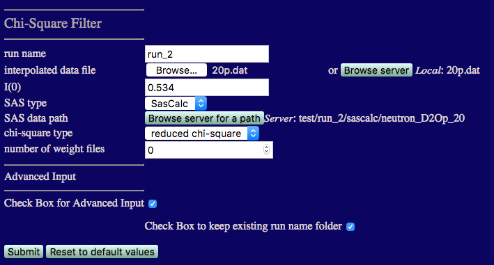
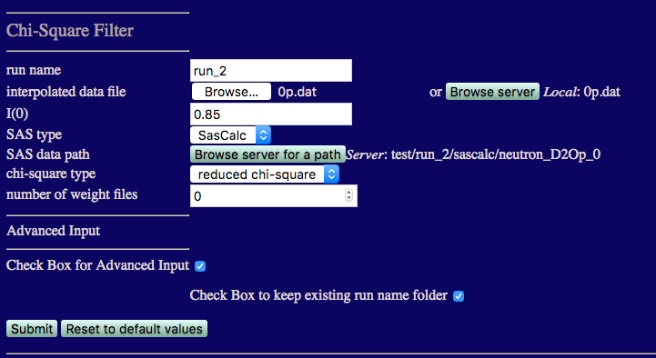
We now repeat the above analysis for the 0% and 20% D2O contrasts. The inputs and outputs are shown below.
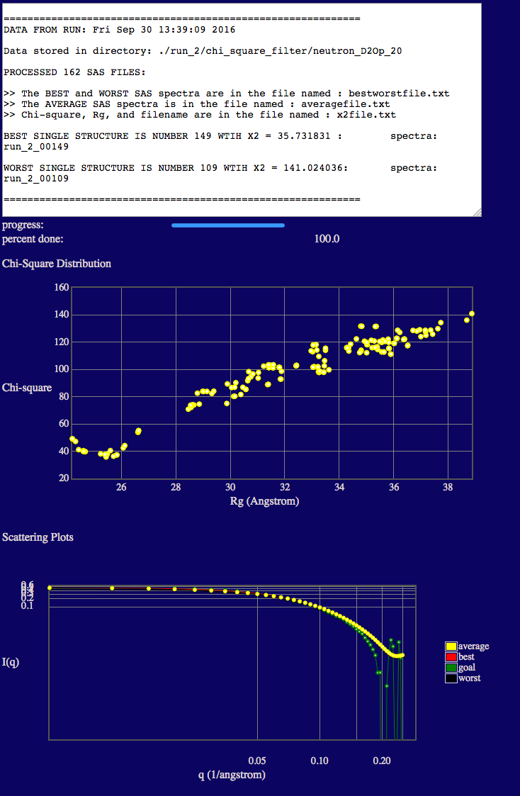
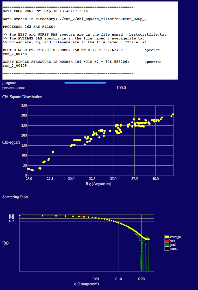
NOTE that the best fit structures for 20% and 0% D2O have higher x2 values than those for 85% D2O. This is because the structure of PAI-1 is fixed and its Rg value is about 2 Å smaller than that found in our contrast analysis. Since PAI-1 is the main contributor to the scattering at these two contrasts, changes in VN structure are not enough to compensate for the Rg mismatch in PAI-1. Better x2 values may be able to be obtained by performing MD simulations or normal mode analysis (ProDy) on the PAI-1 portion of the complex to determine if conformations with slightly higher Rg values can be found. This Chi-Square Filter analysis can then be performed again on the new PAI-VN structures.
test/run_2/chi_square_filter/neutron_D2Op_85
/spectra
test/run_2/chi_square_filter/neutron_D2Op_20
/spectra
test/run_2/chi_square_filter/neutron_D2Op_0
/spectra
We now repeat the above SAS curve comparisons at all 3 contrasts and create a weight file that flags those structures with the best x2 values in each case.
We start with the 85% D2O case. The inputs are shown in the figure below.
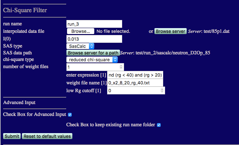
run name run_3 to avoid overwriting earlier calculations
I(0) must match that from the 85% D2O data: 0.013
number of weight files: 1
enter expression[1]:
(x2 < 8) and (rg < 40) and (rg > 20)
weight file name[1]:
Check the box for Advanced Input and then check the box to keep existing run folder name.
The outputs are the same as before except that the desired weight file has also been created.
We now repeat the above analysis for the 0% and 20% D2O contrasts. The inputs and outputs are shown below.
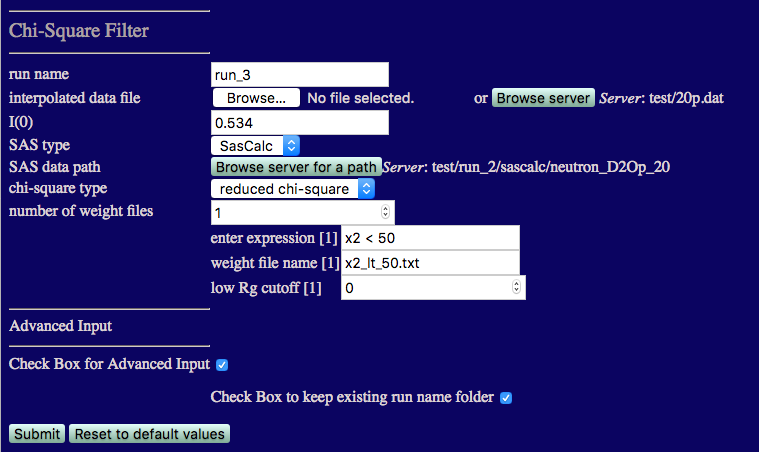
number of weight files: 1
enter expression[1]:
x2 < 50
weight file name[1]:
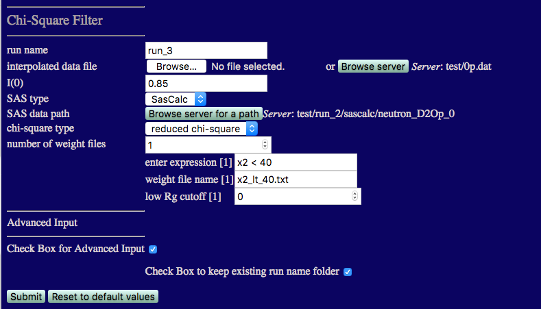
number of weight files: 1
enter expression[1]:
x2 < 40
weight file name[1]:
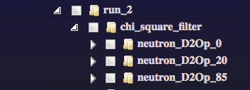
test/run_3/chi_square_filter/neutron_D2Op_85
/spectra
test/run_3/chi_square_filter/neutron_D2Op_20
/spectra
test/run_3/chi_square_filter/neutron_D2Op_0
/spectra
Now, we want to create a single weight file that flags only those structures that are flagged in ALL 3 weight files that we just created. Thus, only those structures that are in the lowest x2 region for all 3 contrasts will be chosen.
An easy way to create this file is to take the average value of the weight flag for each structure from the 3 weight files. If the average value is 1, then the flag is 1 at all 3 contrasts. Otherwise, the average will be a value between 0 and 1. A Python program to perform this average can be downloaded below or you can use your favorite program to perform the average and write out a new weight file.
Now we can filter out the best fit structures for all 3 contrasts and vizualize them using the Extract Utilities. More information can be found in the Extract Utilities documentation.
We will extract the frames from 0_x2_8_20_rg_40.dcd that are flagged in new_weight_file.txt.
The inputs are shown in the figure below.
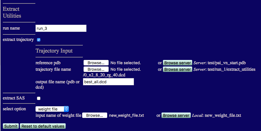
output filename: best_all.dcd
Choose 'weight file' from the 'select option' listbox.
When the process is finished your output should look like the one below.
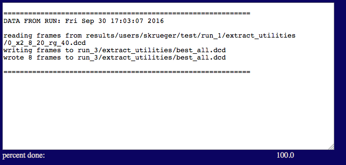
NOTE that there are only 8 frames that satisfy our criteria for this small sampling of structures. In a real study, several hundred to several thousand structures would be needed to adequately define the best fit ensemble for all 3 contrasts.
test/run_3/extract_utilities
The molecular (contrast-independent) Rg was calculated for each subunit, as well as the CM distance between the subunits, for each of the 8 best fit structures.
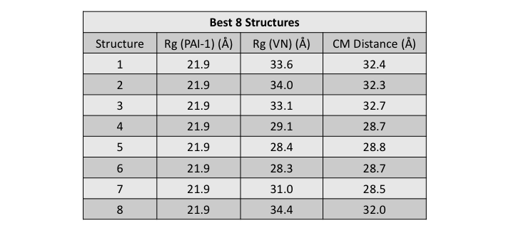
The Rg values for VN are in good agreement with the value found from the contrast analysis. The Rg value for PAI-1 is about 2 Å smaller than the value found from the contrast analysis as previously discussed. The CM distances in these structures are larger than the value of 18 Å that was found from the contrast analysis. This further suggests that our sampling hasn't fully covered configuration space since there should be structures which can satisfy this criterion.
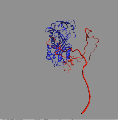
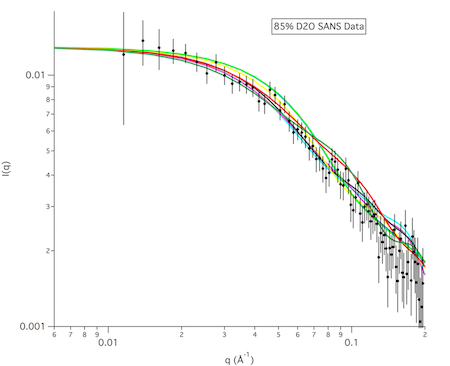
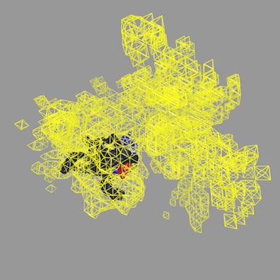
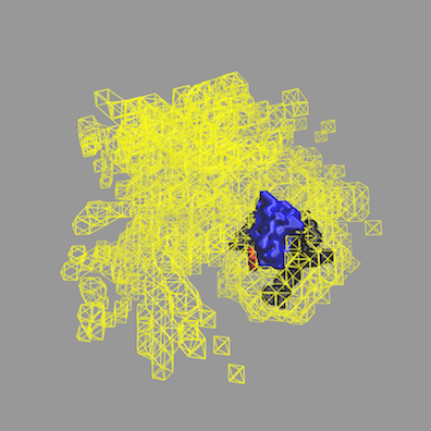
The structures in any of the generated DCD files can be visualized by loading the DCD files along with a suitable PDB file (pai_vn_start.pdb) into VMD. The figure on the left below shows the 8 structures in this example that best fit the data at all 3 contrasts. The figure on the right shows the calculated scattering curves for these 8 structures compared with the 85% D2O SANS data.
Another way to visualize the structures is to use the Density Plot module. The density plot below shows two views of the envelope sampled by all of the accepted structures as well as that sampled by only the best fit structures for all 3 contrasts. The blue and red regions are the envelopes represented by PAI-1 (blue) and the fixed portion of VN (red). The black and yellow regions represent the envelope sampled by the flexible portion of VN for all accepted structures (yellow) and for the best fit structures at all 3 contrasts (black). It is clear from the view on the right that there are portions of configuration space that have not been covered in this limited sampling since there are no yellow or black surfaces covering the blue PAI-1 region.
More information on how to use the Density Plot module can be found in the Density Plot documentation.
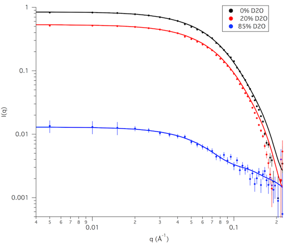
Finally, the figure below shows the calculated data for the single structure from our small sampling that best fits the data at all 3 contrasts (structure #4) along with the interpolated SANS data at those contrasts.
Reminder: This example has only 698 accepted structures and only 8 structures that are in the lowest x2 region for all 3 contrasts. For a real study, 10,000 to 50,000 accepted structures would be needed to better sample configuration space. This would hopefully allow us to find a wider range of structures that best fit the data at all 3 contrasts.
Supported via CCP-SAS a joint EPSRC (EP/K039121/1) and NSF (CHE-1265821) grant